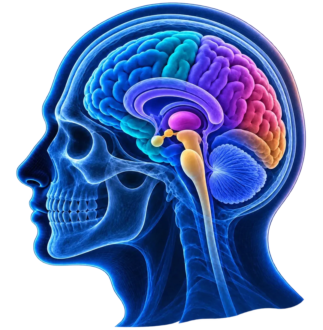
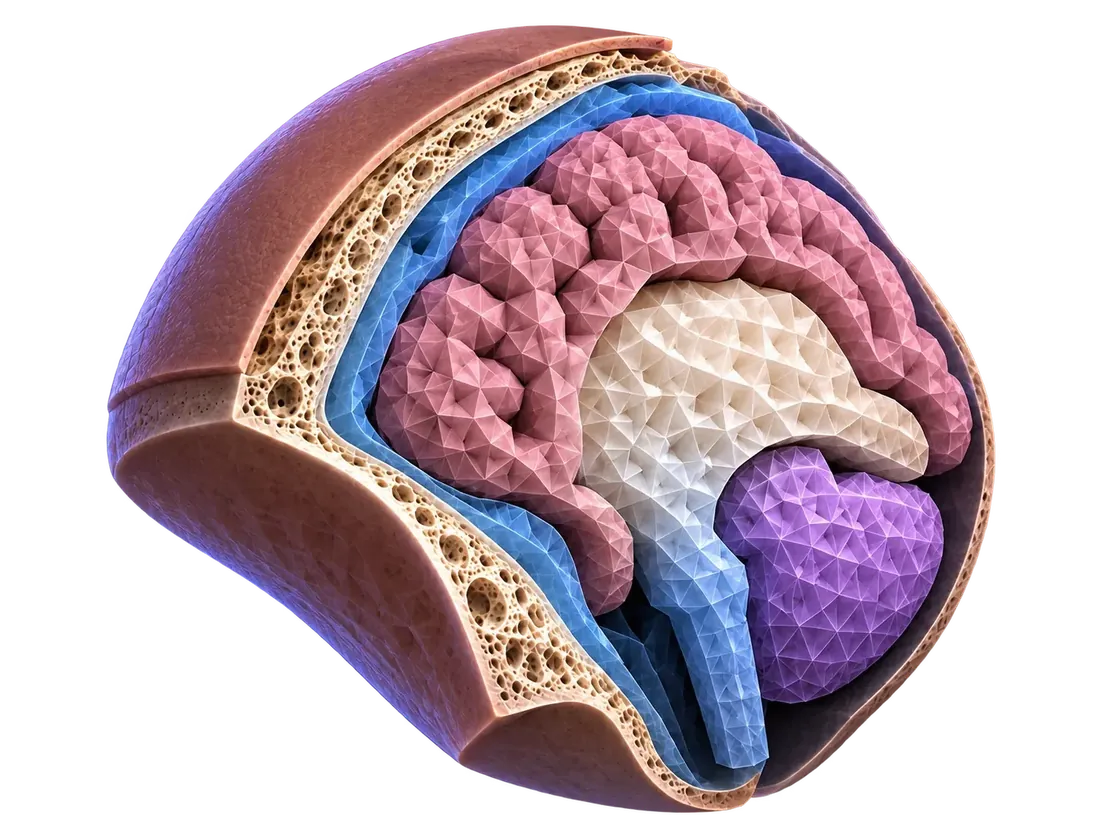
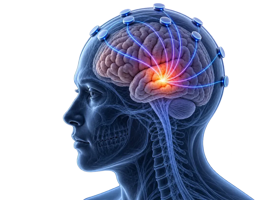
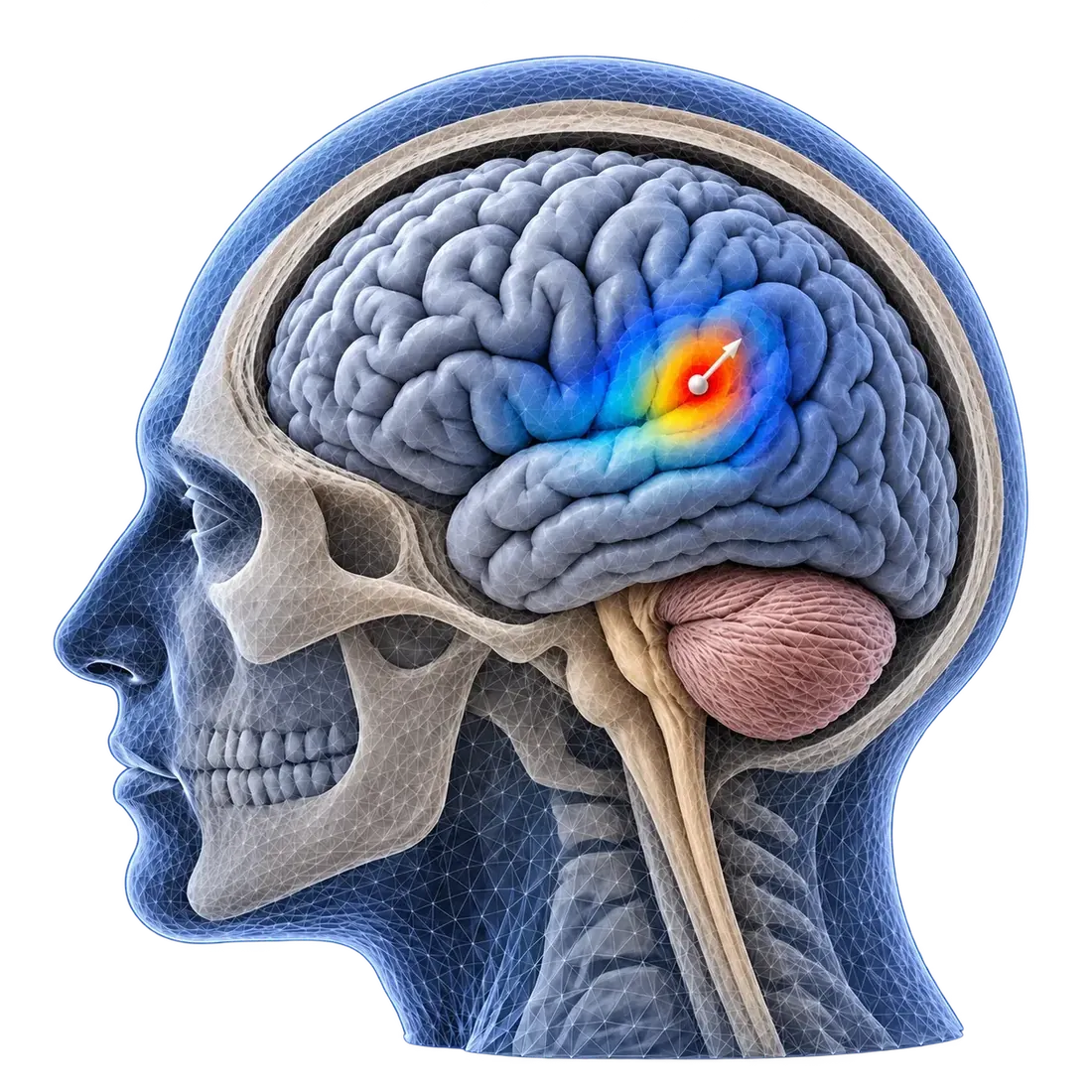
Zeffiro Interface is MATLAB software for a realistic head: closed tissue surfaces,
a labeled tetrahedral mesh, conductivity, sensors, and a lead field
zef.L. Inverse methods then estimate sources from measurements.
This page describes capabilities that exist in the tree — not a product checklist.
01SurfacesImport a .zef segmentation. Compartments, not a volume yet.
02TetrahedraCreate FEM mesh fills the interior and writes nodes / tetra.
03Lead fieldAttach sensors and assemble L for EEG, MEG, EIT, or TES.
04SourcesChoose a rule for y ≈ Lx. Write zef.reconstruction.
01 — Anatomy
Compartments first, volume later
A session starts from closed tissue surfaces. The bundled demo is FreeSurfer-style
.asc files plus a manifest at
data/segmentations/multicompartment_head_project/import_segmentation.zef.
After import, the Segmentation tool lists compartments (scalp, skull, CSF, …).
zef.nodes and zef.tetra stay empty until you mesh.
Each compartment has an activity flag. Sources are placed only where
_sources is constrained or unconstrained field. Inactive tissue,
active surface, and a bounding-box / PML layer are separate states — they are
not interchangeable.
utilities.fs2zef.run — FreeSurfer volumes → surfaces and a .zef
utilities.sn2zef.run — SimNIBS tissues → STLs and a manifest
utilities.brainstorm2zef.run — Brainstorm protocol → live Zeffiro project
utilities.duneuro2zef — DUNEuro MATLAB project → native mesh/sensors/lead field (Open project detects these files)
The converters write anatomy. They do not assemble a lead field. There is no
generic DICOM-to-mesh button in src/io.
Mesh tool → Create FEM mesh runs
zef_create_finite_element_mesh. Closed surfaces are filled with a
Cartesian lattice (five or six tets per cube), then labeled by tissue.
Optional refinement, Taubin smoothing, and a PML lattice when a compartment
is marked as bounding box.
Conductivity is per tetrahedron: isotropic sigma(:,1) in S/m,
or an anisotropic tensor in sigma(:,3:8) for lead-field types 6–10.
The DTI Conductivity Tool maps FreeSurfer FA / NIfTI into those columns.
Applying DTI does not rebuild zef.L by itself.
The mesh step does not create the lead field. GPU paths in this repository
are for transfer PCG, some inverse helpers, NSE, and wave — not for tet generation.
Session electrodes are N×3 (point electrode model) or
N×6 (complete electrode model). EEG / EIT / TES FEM does not
take the six-column array as-is: zef_attach_sensors_volume
builds a four-column attachment table. Positions are parsed from
.dat or headered CSV via core.io.electrodes.
zef_lead_field_matrix dispatches types 1–10: EEG, MEG
magnetometers, MEG gradiometers, EIT, and TES, each with an isotropic
and an anisotropic twin. Source columns are Whitney, H(div), or St. Venant
interpolants. Inverse methods only read L; they do not assemble it.
Optional CUDA uses Jacobi PCG on the transfer solve. CPU uses SSOR or
no-fill incomplete Cholesky. Keep source interpolation on, or inverse
code errors on a missing source_interpolation_ind.
n_s ≫ n_e, so many source vectors fit the sensors. Every inverse
method in this repository is a rule for choosing one x. Both
tracks write zef.reconstruction. They do not share solver code.
Inverse-tools menus labelled (class solver) call
zef_inverse_run and construct inverse.*Inverter.
Other Inverse-tools entries still run plugins/* iterations.
Scripts and cluster jobs should use registry ids, not GUI callback names.
Weighted MNE; dSPM / sLORETA / SBL on a minimum-norm backbone (CSM);
eLORETA’s reweighted filter; LCMV / UNG beamformers; dipole-scan goodness of fit.
Fast when you want a distributed or scanned estimate from L and a frame of y.
Hierarchical Bayesian
IAS MAP with gamma / inverse-gamma hyperpriors. RAMUS averages IAS over
random sparse source subsets at several resolutions — the route aimed at
concurrent cortical and deeper activity when those compartments are active.
Sparse maps
Group Lasso and HALpR (hierarchical Lp) via the EXP optimizers. Use when
the scientific question wants few active groups or a heavy-tailed prior,
not a smooth minimum-norm smear.
State-space
Class Kalman (KF / sLORETA-KF / EnKF, optional RTS). UKF-NMM: spatial Kalman
on a modified lead field, then Jansen–Rit neural-mass parameters with an
unscented Kalman step. DTI structural process-noise Q exists
only on the legacy Kalman plugin, not on inverse.KalmanInverter.
After a reconstruction, inverse.gmm can cluster the map. That is
not itself a registry inverse id. Kalman / UKFNMM share predict–update kernels
in inverse.kf.
05 — Observe
See the mesh, the map, the traces
The Figure tool owns the 3-D axes. Mesh visualization draws volume and
surfaces, clipping planes, and cameras. After an inverse, colour the tetrahedra
from zef.reconstruction. Overlays include cones, contours,
DTI streamlines, and source markers.
Time is first-class: frame sliders, movie loops, a butterfly window, and
parcellation time series when an atlas or user spheres have been painted
onto the source space. Measurements and reconstructions import as
.mat / .dat — not as native EDF or FIF.
The whole session is the zef struct. zef_save /
zef_load persist scientific fields (handles stripped). Scripts
call the same functions the buttons call, including
zef_inverse_run(zef, 'eloreta', 'execution', 'local').